Digital twins for live petroleum production optimization

A high-frequency live connection to data feed from sensors on equipment offers several benefits such as facilitating human surveillance for better asset management, identification and diagnosis of abnormalities and suboptimal operation. However, normal operation does not necessarily imply optimal operation.

To obtain optimal production, the asset must be operated at appropriate setpoints. For dynamic assets or systems, the optimum setpoint changes with time. In such cases, the live data feed associated with the equipment’s Industrial Internet of Things (IIoT) network can be harnessed to develop a dynamic setpoint optimization mechanism.

Existing literature on petroleum production optimization on artificial lift wells setpoints is focused on manual simulation, design and recommendation by experts, or through semi-automated batch implementation of evolutionary, [1] statistical or machine learning (ML) models. Current literature on digital twin implementations [2] in oil and gas present a broader picture on overall production process optimization [3], but not on dynamic individual asset level set-point optimization. Fully automated set-point recommendation requires a data processing engine integrated with a simulation engine that can manage, process and generate large volumes of data.

Digital twins representing systems of assets can be valuable in determining optimal operating set-points. The integration of live IIoT data-feed with a digital twin system offers several challenges and requires a detailed design for effective implementation. The following aspects of the implementation are detailed in this paper: Data processing: profiling, clean-up, transformation and cloud-database maintenance for multiple assets, high frequency data Simulation: Automated cloud-database triggered field data relevant massive scale simulation (60,000 + per day).

The specific use case chosen in the paper for showcasing the methodology is related to set-point changes on the artificial lift[4] equipment of the well for optimizing the production system.

Digital twin schematic

The design and implementation of a digital twin for dynamic set-point optimization on a petroleum production system using live IIoT data consists of several steps. These are:

1. Field data processing: Collection, profiling, clean-up, transformation and cloud-database maintenance
2. Simulation: Automated cloud-database triggered field data relevant simulation
3. Inverse modeling, which consists of:
   1. Connecting real-world IIoT data with simulations to learn system unknowns
   2. Evaluation: Estimate how closely the digital twin mimics the real-world asset from history
   3. Calibration: Implement initial steps using insights from digital twin to account for uncertainty
4. Artificial intelligence (AI) model recommendation: Deploy automated recommendations for set-point adjustments with updates based on dynamic trending of the asset.

This article focuses on the automation of the first two items of this process: Data processing and simulation. These steps are described in the context of feeding an AI engine that further consists of inverse modeling and model generated recommendation system. The details of the Inverse modeling and AI model recommendation components are beyond the scope of this paper.

Figure 1 represents a schematic of the overall process. It is important to note that this is a closed-loop ongoing process and not a feedforward sequence of steps that ends in a recommendation. This distinction is important for two main reasons:

1. After a model-generated recommendation has been implemented, a digital twin that is a live virtual representation of a physical system needs to identify changes in operating state, record and evaluate the response and trigger an ongoing cycle involving data processing, simulation, inverse modeling to adjust the system in case if the provided recommendation needs to be followed up with a new recommendation.
2. The digital twin can evaluate the impact of all historic set point changes and fine-tune the recommendation system.

Figure 1: Schematic of the closed-loop process providing an overview of the digital twin. Courtesy: Industry IoT Consortium

The current state

Before going further into the details of the digital twin implementation, it is necessary to understand the scope and potential impact by describing the typical current state of operation in the oil and gas industry.

The process described in Figure 1 is already widely in the oil and gas industry. However, every step in the process is performed manually by subject matter experts (SMEs) on a well-by-well basis. The manual process is time-intensive, it takes several hours to implement it on one well for data collection, processing, simulation, inverse modeling and generating a setpoint recommendation using a history matched model. Petroleum wells are dynamic entities that change their underlying operating conditions over time.

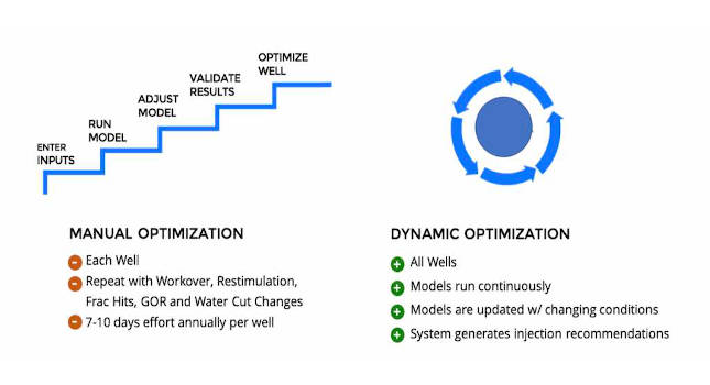
Further, wells are subjected to discontinuities in behavior due to design changes, workovers, re-stimulation and impact from nearby operations such as hydraulic fracture hits. Setpoint reviews or changes are required as the well behavior changes. If diligently performed, the time investment required to optimize setpoints is approximately 7-10 days per well per year. Due to the significant time investment, typically, the simulation-based setpoint optimization is employed semi-annually or annually per well, or when there has been a redesign or a workover. The details of the typical procedure are represented in the manual optimization section of Figure 2.

The automated version of the manual optimization results in dynamic optimization. Such a system can go through the entire process from data collection through to setpoint recommendation for all wells on a continuous basis. Changes in well operating states are programmed to be detected, and the underlying models that are used to generate the setpoint recommendations get updated with changing well conditions.

The term “automation” in this paper refers to the implementation of a system designed to minimize human intervention by identifying, templatizing, storing, scheduling and executing repeatable processes. While it is feasible to generate manual setpoint recommendations, manually updating and generating simulations every time there is a change in the system for a field consisting a few hundred wells is intractable. Thumb-rules or intuition-based setpoint optimization takes the forefront position when compared to physics-based-modeling.

The scope and intent of this paper is to describe a system capable of automating massive scale simulation and the associated data processing using a cloud based distributed system. Such a system stores, transfers and processes data, and subsequently queues, executes and stores the results from thousands of simulations relevant to several hundreds of wells on an ongoing basis.

The expected impact of the paper is to provide motivation to set up pipelines for automating components or entirety of the data processing, simulation, inverse modeling and setpoint recommendation workflow in the oil and gas industry and other analogous spaces capable of utilizing an IIoT network for developing a digital twin as defined in the introduction section of this paper.

Figure 2: Comparison between manual optimization (current state) versus dynamic optimization that can be achieved through the digital twin. Courtesy: Industry IoT Consortium

Data collection

The first component of our digital twin as described in Figure 1 is: Field data processing. Field data contains variety, Figure 3 highlights this variety through some examples.

Regarding field data, there are two primary types: Sensor data and metadata.

1. Sensor data: The live signal from various sensors on assets was collected by a supervisory control and data acquisition (SCADA) system. Some general examples of sensor data include:

• Pressures, flow rates, temperatures for the well site, surface facilities and well downhole.
• Other examples specific to artificial lift equipment may include details such as: Pump frequency, voltage, compressor discharge and intake pressures.

Figure 3: Data variety – sensor data, metadata. Courtesy: Industry IoT Consortium

These sensor signals were collected through wellsite telemetry and dropped onto a cloud-based storage by the well operator’s SCADA provider. This data was typically accessed by the operator for monitoring and surveillance. The sensor data is universally accessible once access credentials are shared for data transfer. Such data is time-series data and is typically transferred in files titled after a time-stamp and containing the sensor signal for all the assets during a chunk of time. It might be worth noting that the sensor streams can be intermittent due network or telecommunication issues, delivered out of order or on a time delayed basis. These time-specific files can be aggregated and restructured to tables as suited by the user. In this case, this data was converted to tables indexed by asset ID and timestamp, with corresponding sensor signals stored in columns. An example of such a file is displayed in Figure 3, in the image titled “Sensor Data: Flat files – csv.”

2. Metadata: To further represent the system which the sensor data is associated with, the metadata of the system is necessary. Examples of metadata can include but not restricted to:

• Name, location, deviation and completion data of the well
• Design data for the artificial lift equipment
• Piping and instrumentation schematic of the well and facilities sites
• Fluid properties: Pressure, volume and temperature (PVT) data.

Figure 3 highlights how the metadata may be available in various formats such as images, excel sheets, PDF documents etc. A key component of automation is to digitize the various forms of data into a uniform data store. This involves creating a template that records the quantitative details of the metadata. An example of such a digitized template of the metadata is displayed in Figure 4. Once digitized, metadata is extractable through an API as a hierarchical data format such as JSON.

It is important to note that metadata is not usually available at a single location or from a single source. There is a significant amount of manual effort that goes into contacting the field operators, the SCADA company, the equipment manufacturers to gather this data and to digitize it. A uniform reference data store space was created on the cloud to maintain and access the raw metadata as a source of truth.

Metadata is often manually entered into the system because it is associated with the well when it is installed and does not change afterwards. When there is a maintenance event that changes a physical equipment of the well, the metadata may need to be updated depending on the changes being performed.

Figure 4: Template for digitized well metadata. Courtesy: Industry IoT Consortium

Data processing

The sensor data and metadata were recorded and digitized from various sources. Further the data processing steps after this includes:

• Mapping data
• Profiling
• Cleanup
• Transformation
• Labeling events
• Flagging changes.

Mapping: As described in the previous section, sensor data and metadata come in different formats and are stored in different formats. Similar devices from different providers or SCADA systems often have different naming schemes, these sensor tags need to be mapped to their appropriate devices and assets. After the name mapping the time series sensor data is mapped to its asset metadata by merging the two data sources by asset ID.

Data profiling: After mapping sensor data and metadata, sensor data will be going through an exploratory data analysis (EDA) process which we call as data profiling step. In this step, we look into some specific properties of well’s sensor data to determine if it meets our model’s requirements and we can create a cohort of wells which have sufficient data properties to be used in our models. Those properties are including but not limited to monitored time, lapse time/monitor time ratio, zeros ratio and frequency.

Monitor time quantifies how much historical data that a well has. Lapse time is defined as a period where we don’t receive any signal from the well, therefore lapse time/monitor time ratio is to determine the proportion of data availability over the life of a well. Zeros ratio is used to see the actual variance in data. Frequency of data is also a key factor to the success of our models, the more granular data we have the better our models’ performances are. A set of thresholds will be applied on each of the properties mentioned above. Sensors that meet these thresholds will be examined to see if they are sufficient for our models. Wells that include these qualified sensors are included in a cohort.

An example of monitored time threshold is shown below where monitored time threshold is set at 90 days which consequently reduces the number of wells in the cohort from 217 to 56 wells.

Figure 5: Cohort selection based on monitored time. Courtesy: Industry IoT Consortium

Cleanup: Data coming from several wells may include various challenges such as abnormal states of operation of the well (for example: shut-in, maintenance job, inconsistent performance), faulty signal, signal lapses, signal names that are inconsistent from convention. It is necessary to identify these inconsistencies. Some of these can be identified and eliminated systematically, such as identification of dummy values of a signal, removal of outliers, or identifying that a well is shut in. There are other abnormalities that require human review, for instance, a signal that was named inconsistently, or a metadata element that does not fit the template.

Transformation: It is not beneficial to evaluate meaning out of data or generate simulations at the frequency of live data. Signals may be recorded at different timestamps and variable frequencies. In the work presented in this paper, data was resampled to a daily frequency to match the frequency of the production rates of the wells. Further, the variation related features such as the oscillation frequency/wavelength, level of stability when compared to the normal signal was captured through a rolling normalized coefficient of variance. Unstable states were treated separately from stable states of operation. Figures 6 and 7 represent the use of box plots, and normalization of data, for outlier detection and identification of stable states.

Figure 6: Box plots indicating distribution of change in measured variables due to setpoint (gas injection rate) changes. Courtesy: Industry IoT Consortium

Figure 7: Identification of stable operating states through normalization. Courtesy: Industry IoT Consortium

Labeling events: When assets undergo gradual or prolonged states of abnormal behavior, the normalization filters may not be sufficient to identify and isolate such time zones. A monitoring platform that facilitates labeling can be a great tool. In the use case presented in this paper such a platform was used for Identification of events of interest by subject matter expert review. This method can be fast, effective and multipurpose. Data associated with the timestamps of the label can be easily extracted and utilized for further analysis, and supervised machine learning models can be trained for detecting such complex anomalies. [5] Figure 8 shows an image of such an expert reviewed label to identify abnormal time.

Figure 8: Labeling of abnormal events. Courtesy: Industry IoT Consortium

Flagging changes: To have a closed loop system for generating setpoint change recommendations, it is imperative record historical and life setpoint changes in the system to identify and evaluate the response to the stimulus. An illustration of recording flagging changes and their responses is presented in Figure 9. The gas injection rate displays the set point value, oil and water sensors represent the responses measures to a setpoint change. In Figure 9, the periods across setpoint change indicated by greyed zones are marked such that tubing and casing pressures are operating in a stable state. Measuring the response of a set point change while the well is operating abnormally leads to incorrect evaluation.

Flagging changes has its similarities and differences when to identification of abnormalities. The difference is that abnormalities are usually not human controlled and are usually unintentional. The similarity is setpoint change and abnormalities indicate a change in operating state. These can be identified through supervised methods such as labeling followed by machine learning models, and unsupervised methods such as measuring deviation beyond a threshold. The approach in this paper is a supervised “human-in-the-loop” approach, where setpoint recommendations generated by the system are monitored and reviewed by the operator prior to implementing the change. This is also a step towards expert augmented machine learning [6], where the feedback provided by the expert on the model generated recommendations is utilized to adapt the model to provide improved recommendations in subsequent rounds.

Figure 9: Flagging changes and recording the response to the stimulus. Courtesy: Industry IoT Consortium

Simulation of virtual data

Having covered the collection and processing of physical data, in this section we proceed to describe the methodology for automated generation of virtual data. Simulation represents the virtual data generating component of the digital twin. The oil and gas optimization literature is rich in description of simulation based artificial lift and gas lift setpoint optimization approaches. The paper by Rashif et al. [7] summarizes a survey of different gas lift optimization techniques using simulation. Borden et al. [8] presented a surveillance and workflows-based approach for gas lift optimization. Surendra et al. [9] presented further progress in the field by automating combining the analytics and physics-based modeling/simulation approaches through a case study in a Middle East oilfield, this study included the approach to simulating 50 wells in less than two weeks’ time.

The work presented in the current paper takes a step further any creates a live-connection between field IIoT sensor data and a cloud-based simulation system that can generate 60,000+ simulations per day taking input from field data. This coupling between the physical and virtual data represents a key component of the digital twin. An effective digital twin is expected to represent and mimic a physical system. Hence, the simulation scheme described is closely connected to the physical data to maintain relevance.

The simulation section covers the following topics:

• Simulation schematic
• Simulation input
• Simulation output.

Simulation schematic:

A commercial transient physics-based simulation software was employed to represent the fluid flow from the oil and gas reservoir through wellbore and the surface facilities that include the separation system and pipelines to transport fluids.

Figure 10 represents the process flow diagram of the physical setup and its corresponding simulation setup. Well and surface facilities schematics may vary among operators, fields, even between well pads. To generate a new exact simulation schematic for every variation in physical process flow is a very time-intensive process.

For templatization purposes, the simulation scheme has been simplified to include only those components that are relevant to the objective. For example: in the process flow diagram in Figure 10, there are multiple tanks per fluid, this is reduced to a single tank per fluid in the simulation schematic since the back pressure created by the downstream tanks is negligible.

However, the templatization process can in some cases also add complexity to the system. For instance, the process flow diagram in Figure 10 represents a single well system with no connections to other wells. However, the corresponding simulation schematic includes a gas source coming from other wells downstream of the separator. This complexity has been included to make the simulation template a general one that can be utilized on systems with gas lines commingling from multiple wells. In the case of a single well system, the parameter’s value is set to zero.

Figure 10: Field data process flow diagram and its corresponding simulation schematic. Courtesy: Industry IoT Consortium

Simulation parameter sensitivity was assessed using box plots similar to the examples shown in Figure 6. It was observed that the spread of change (0 to 30 psi) in separator pressure was higher than that of bottom-hole pressure (0 to 3 psi) during setpoint changes. This exploratory data analysis was helpful in the design of the simulation setup that led to some crucial decisions. For example, reduction of bottom hole pressure is considered one of the primary objectives [10] of artificial lift. In the nodal analysis performed through simulation software it is common to find literature with separator or the wellhead specified to be the end node [11].

Such systems assume the end node pressure to be constant during a setpoint change. In a previous version of this work, several challenges were observed in mimicking the out pressures of physical system due to the assumption that the simulated wellhead/separator pressures were to be held constant during a gas injection change. Based on the data from the box plots, it was demonstrated to be an incorrect assumption.

To mimic the physical system that accommodates separator pressures to change with changes in gas injection rates, the gas sales and compressor nodes downstream of the separator were set to be the end nodes. This resulted in a better correlation between simulation output and physical sensor output during gas injection changes.

Simulation input:

The simulation schematic shown in Figure 10 is a graphic user interface (GUI) representation of a simulation file of the commercial physics-based simulator, such as Ledaflow or Olga. Each GUI based case has an associated input file that can be broadly divided into:

1. Static parameters: Inputs that are fixed for the entire run of the simulations, such as the well completion and design data, reservoir fluid properties, pipeline and separator properties.
2. Dynamic parameters: Inputs that can vary as a function of time such as the gas injection rate, reservoir pressure, produced gas to liquid ratio and water cut, sales gas back pressure, other wells gas.
3. A system has been set up to write simulation input files based on the parameters obtained from a queue of simulations stored on a No-Sql Database such as MongoDB or PostgreSQL. The architecture of this system is further elaborated in a subsequent section.

Simulation inputs are queued on the No-Sql Database based on the type of parameters as described in Table 1. The parameters described in the “knowns” section in Table 1 are recorded from field data. These parameters are updated in the simulation queue based on timely trends in field data. The value of these parameters is based on the exact operating range observed in the processed field data. The “unknowns” correspond to parameters whose values are difficult to measure yet have a significant sensitivity.

These may include static parameters such as the tubing friction factor, or dynamic parameters, which vary at a high rate. Since the input values for these parameters are unknown, a wide range of possibilities within the bounds of physical guardrails are input for these parameters. The “approximations” column in Table 1 refers to parameters that have some sample data from the field, but not precise, live, or well-specific data. These parameters can be approximated within a smaller range because of their static nature and relative insensitivity.

The simulation queue consists of combinations of the known, unknown and approximate parameters. New simulations are added to the queue based on the rate of change of the field data. After a point of time, further simulation may not be necessary on a well, as historical simulation may have covered the operating range. The ranges of the unknown parameters also narrow down with time as the inverse model provides estimates based on history matching.

Table 1: Details of simulation parameters and relationship to field data. Courtesy: Industry IoT Consortium

The commercial physics-based simulator employed in the case presented is a transient simulator. This implies that some of the input parameters can be entered as a time series, and the response to changes in these parameters can be obtained as a time series output. This detail is a key component of the simulation setup because the startup of a simulation and the post-processing associated with writing outputs to files has a non-trivial overhead on the simulation schedule. To reduce the input-output overhead and transition associated delays between simulations, dynamic parameters such as Reservoir pressure, Productivity index etc. are stepped through time series.

In the current case, 240 simulation cases were connected together as a time series, and input into a simulation queue as a single item. Each item read from the queue generates a commercial simulator input file with 240 cases in series. The number of cases per simulation file has been heuristically arrived at as an optimum scenario. If a very large number of cases are input per file, that may overload the system memory and output large files, this may lead to a system crash. A smaller number of cases input per simulation file results in underutilization of the transient capabilities of the simulator, and loss of time in the simulation input-output process.

Simulation output:

Each simulation file generates a time series output for the 240 cases as described in the simulation input section. The simulation output is updated to the No-Sql database item associated with its input. Python scripts are set up to extract the data from a No-Sql database, and post-process the time series data and extract individual case outputs corresponding to each input. These simulation outputs are matched with field observations to identify simulations representing likely operating states of the well. The “unknown” parameter values in simulation cases associated with output values irrelevant to field data are disincentivized in further rounds of simulation as a part of the inverse modeling process. A rough visual representation of the response comparison between field data and simulation is presented in Figure 11.

Figure 11: Response comparison between field measurement and simulation output. Courtesy: Industry IoT Consortium

In the use case presented in this paper the response variables being matched with field data include:

• Oil production rate
• Wellhead pressure
• Downhole pressure.

In the inverse modeling process subsequent to the simulation, further constraints are implemented on the relationship between simulation output and field responses including the historical trends that identify the likelihood of a combination of unknown parameters. Thus, the operating state of a well at a given time is estimated through this process, and this knowledge is used to generate setpoint recommendations.

Live sensor data processing:

Live sensor data processing starts with sensor data being added to an on-cloud source location where it can be read by a monitoring workflow system. The monitoring workflow system copies the newly-changed files and starts the extract, transform, load (ETL) process. The system often starts with a scheduling system, which allow for workflows to be written as directed acyclic graphs (DAGs) of tasks. The scheduler executes these tasks on multiple workers following the specified dependencies between tasks and can be elastically scaled depending on load.

The ETL processes act as producers in a common messaging system workflow. The ETL process adds encoded sensor values as messages to a queue to be later read by consumers which store the data into a time series database. Processing queues create distributed durable queues for processing of queued data. Individual queue consumers can have purpose developed functionality for persisting sensor streams, creating new values and derived or calculated sensors.  These durable queues provide a significant buffer of messages to be added if there is a spike in demand and consumers are not able to keep up with producers.

Eventually, the time series based sensor stream needs to be persisted in a time series aware storage system. These time series storage solutions are purpose built data stores that store and query temporal data. Some of these stores can scale to millions of operations per second. Having a time series or temporal query engine becomes critical to process sensor streams.

The system design allows for reprocessing of data if needed. The repeatable transformation process allows for better recovery from errors and bugs. The system is also performant. It is not uncommon to process 600k sensors per minute and the system can also scale to higher throughput by adding workers, queue partitions, or database nodes.

Simulation workflow

After data processing, it’s time to use the data to generate simulation cases. The data is analyzed for parameter ranges to explore in simulation. Simulation cases are partitioned by field data and queued in a document database collection. Cloud instances configured with the commercial simulator software and a Python process consume the queue and process cases. Our commercial simulator can be called using a command line interface using a JSON file for input. The output from the simulator is saved to the same document with the case and the status is marked as completed.

A single simulation generates 63 MB of uncompressed data and 467 data points (approximately 4 TB of data per day). However, our inverse modeling process requires only 40 of those data points and we use compression to store the portion of the results needed. A single instance of the simulator can process about 15K cases a day (approximately 10 cases a minute). We use 4 instances to process 60K cases a day and this process can be scaled up to more instances if needed.

Conclusion

The typical processes of the oil and gas industry with respect to data processing, simulation for well modeling and artificial lift set point optimization are time-intensive due to their manual nature. With the limitations of number of engineers per well [12], and with high decline rates [13] contributing to highly transient behavior, continuous optimization is a challenge. Inability to update setpoints along with changes in well behavior may result in sub-optimal production rates. There may be significant economic benefit by optimizing setpoints through increase in production, and/or reduction in operational costs [14].

By harnessing live data feed, on-cloud processing power in combination with simulation and data science tools, it is possible to develop a digital twin for scalable setpoint optimization based on physics-based models on fields with hundreds of wells. In the digital twin, there is an interactive system between the field data from the physical world and the virtual data from the simulations. An overall framework for developing such a digital twin has been presented in this paper.

The design and implementation details along with the architecture of the system required to automate continuous field data processing and a massive scale simulation engine that can generate 60,000+ simulations per day has been described. The benefits and challenges in minimizing human involvement for automating key components of the system have been addressed, while also highlighting the components that benefit from a human-in-the-loop. The on-cloud solution also provides an opportunity to scale-up the capacity on an as needed basis by multiplying the computational units.

Several key decisions were made in terms of choosing the architecture for the system, integration with a platform that supports event labeling, factors to consider for templating the simulation setup, and facilitating the simulation output to be compared with field data. The importance and examples of these decisions were presented in the paper to help in adopting and replicating this work.

The methodology and experience shared in this paper is expected to help the community get one step closer to scalable and generalized automated setpoint optimization, and also help engineers free-up their time for important decision making, rather than spending it on templatizable and repetitive tasks such as setting up simulations manually.

This infrastructure live massive scale simulation coupled with field IIoT sensor data paves the way towards the next steps required for closed loop dynamic setpoint optimization.

Venkat Putcha, director of data science OspreyData Inc.; Nhan LeData, scientist, OspreyData Inc.; Jeffrey Hsiung, principal data scientist, OspreyData Inc. This article originally appeared in the IIC JOI. The Industry IoT Consortium is a CFE Media content partner. Edited by Chris Vavra, web content manager, Control Engineering, CFE Media and Technology, cvavra@cfemedia.com.

REFERENCES

[1] Garcia, Artur Posenato, and Vinícius Ramos Rosa. “A Genetic Algorithm for Gas Lift Optimization with Compression Capacity Limitation.” Paper presented at the SPE Latin America and Caribbean Petroleum Engineering Conference, Mexico City, Mexico, April 2012.doi: https://doi.org/10.2118/153175-MS

[2] LaGrange, Elgonda “Developing a Digital Twin: The Roadmap for Oil and Gas Optimization.” Paper presented at the SPE Offshore Europe Conference and Exhibition, Aberdeen, UK, September 2019.doi: https://doi.org/10.2118/195790-MS

[3] Okhuijsen, Bob, and Kevin Wade. “Real-Time Production Optimization – Applying a Digital Twin Model to Optimize the Entire Upstream Value Chain.” Paper presented at the Abu Dhabi International Petroleum Exhibition & Conference, Abu Dhabi, UAE, November 2019.doi: https://doi.org/10.2118/197693-MS

[4] https://www.rigzone.com/training/insight.asp?insight_id=315&c_id=

[5] Pennel, Mike, Hsiung, Jeffrey, and V. B. Putcha. “Detecting Failures and Optimizing Performance in Artificial Lift Using Machine Learning Models.” Paper presented at the SPE Western Regional Meeting, Garden Grove, California, USA, April 2018. doi: https://doi.org/10.2118/190090-MS

[6] arXiv:1903.09731

[7] https://doi.org/10.1155/2012/516807

[8] https://doi.org/10.2118/181094-MS

[9] https://doi.org/10.2118/201298-MS

[10] https://oilfieldteam.com/en/a/learning/gas-lift-28072018

[11] Camargo, Edgar & Aguilar, Jose & Rios, Addison & Rivas, Francklin & Aguilar-Martin, Joseph. (2008). Nodal analysis-based design for improving gas lift wells production.

[12] https://jpt.spe.org/so-many-wells-so-few-engineersscaling-production-engineering-all-those-shale-wells

[13] https://www.hartenergy.com/exclusives/why-us-shale-production-declines-are-higher-you-might-think-188251

[14] Redden, J. David, Sherman, T.A. Glen, and Jack R. Blann. “Optimizing Gas-Lift Systems.” Paper presented at the Fall Meeting of the Society of Petroleum Engineers of AIME, Houston, Texas, October 1974. doi: https://doi.org/10.2118/5150-MS

Original content can be found at Oil and Gas Engineering.

Do you have experience and expertise with the topics mentioned in this content? You should consider contributing to our CFE Media editorial team and getting the recognition you and your company deserve. Click here to start this process.